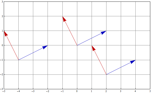
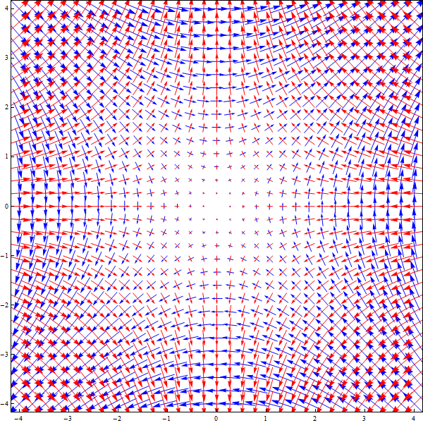
 Similarly for a given vector field
\begin{equation*}
\vec{F}(x,y) = u(x,y) \vec{\imath} + v(x,y) \vec{\jmath}
\end{equation*}
we can consider the vector field which is orthogonal to it
\begin{equation*}
\vec{G}(x,y) = -v(x,y) \vec{\imath} + u(x,y) \vec{\jmath}.
\end{equation*}
Then, calculating the flow lines of these two vector fields will lead to two families of curves which are at each point orthogonal to each other.
Similarly for a given vector field
\begin{equation*}
\vec{F}(x,y) = u(x,y) \vec{\imath} + v(x,y) \vec{\jmath}
\end{equation*}
we can consider the vector field which is orthogonal to it
\begin{equation*}
\vec{G}(x,y) = -v(x,y) \vec{\imath} + u(x,y) \vec{\jmath}.
\end{equation*}
Then, calculating the flow lines of these two vector fields will lead to two families of curves which are at each point orthogonal to each other.
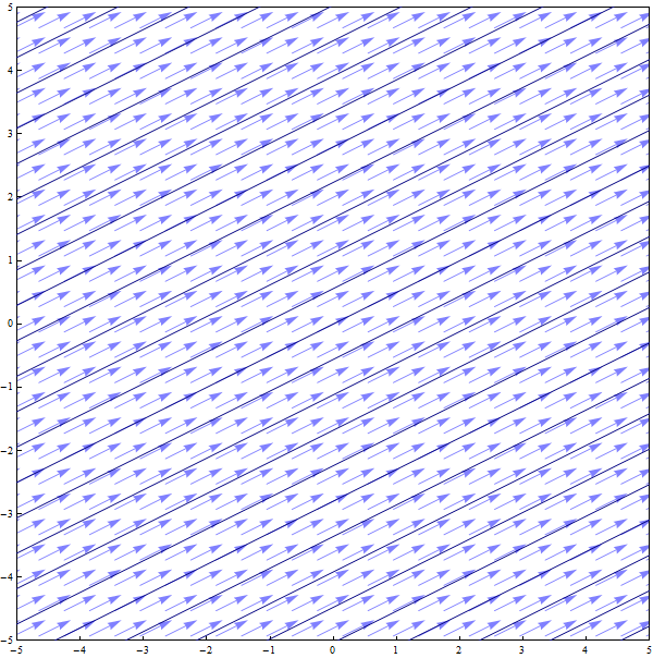
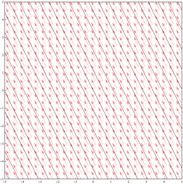
 To get the explicit solutions for the flow lines we have to solve differential equations
\begin{equation*}
f'(t) = 2 \qquad \text{and} \qquad g'(t) = 1.
\end{equation*}
The solutions are
\begin{equation*}
x = f(t) = 2t +c_1 \qquad \text{and} \qquad y = g(t) = t + c_2.
\end{equation*}
Or, eliminating $t$ we have $y = (1/2) x + c$ where $c$ is an arbitrary constant.
To get the explicit solutions for the flow lines we have to solve differential equations
\begin{equation*}
f'(t) = 2 \qquad \text{and} \qquad g'(t) = 1.
\end{equation*}
The solutions are
\begin{equation*}
x = f(t) = 2t +c_1 \qquad \text{and} \qquad y = g(t) = t + c_2.
\end{equation*}
Or, eliminating $t$ we have $y = (1/2) x + c$ where $c$ is an arbitrary constant.
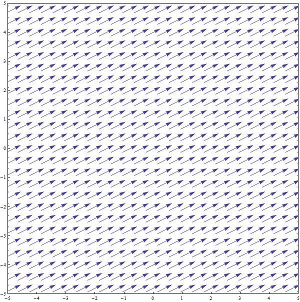
 The orthogonal vector field to $\vec{F}$ is
\begin{equation*}
\vec{G}(x,y) = (-1) \vec{\imath} + 2 \vec{\jmath}
\end{equation*}
The orthogonal vector field to $\vec{F}$ is
\begin{equation*}
\vec{G}(x,y) = (-1) \vec{\imath} + 2 \vec{\jmath}
\end{equation*}
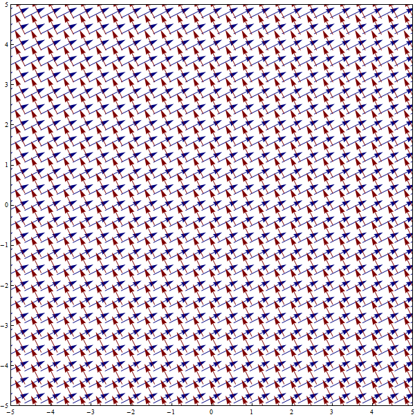 The flow of this vector field consists of parallel lines with slope $-2$.
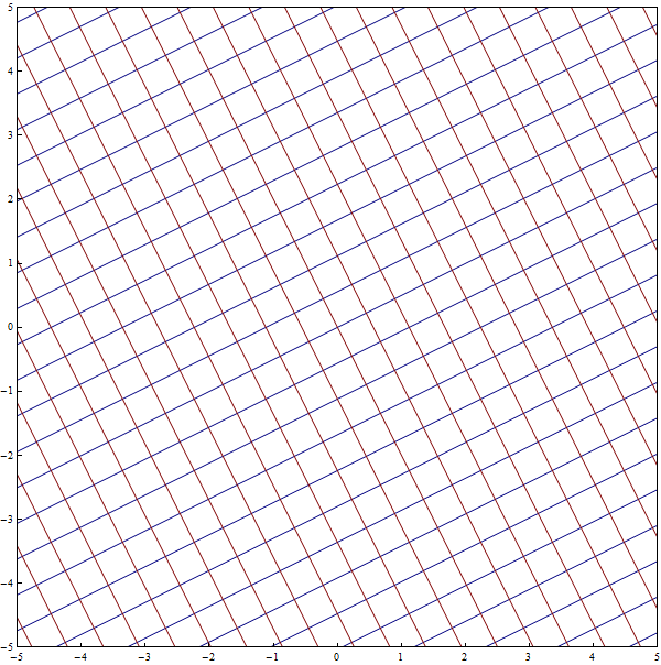
 In this way we have obtained two families of mutually orthogonal lines
 At this point you are asking: What is a big deal? I hope next examples will show that.
 To get the explicit solutions for the flow lines we have to find the parametric curve $x=f(t), y=g(t),$ by solving the differential equations
\begin{equation*}
f'(t) = 1 \qquad \text{and} \qquad g'(t) = f(t).
\end{equation*}
The solutions are
\begin{equation*}
x = f(t) = t +c_1 \qquad \text{and} \qquad y = g(t) = (1/2)t + c_1t + c_2.
\end{equation*}
Or, eliminating $t$ we have $y = (1/2) x^2 + c$ where $c$ is an arbitrary constant.
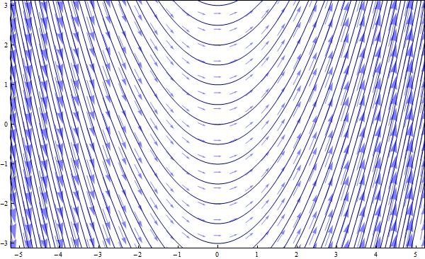
To get the explicit solutions for the flow lines we have to find the parametric curve $x=f(t), y=g(t),$ by solving the differential equations
\begin{equation*}
f'(t) = 1 \qquad \text{and} \qquad g'(t) = f(t).
\end{equation*}
The solutions are
\begin{equation*}
x = f(t) = t +c_1 \qquad \text{and} \qquad y = g(t) = (1/2)t + c_1t + c_2.
\end{equation*}
Or, eliminating $t$ we have $y = (1/2) x^2 + c$ where $c$ is an arbitrary constant.
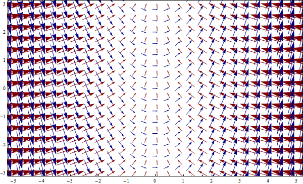
 The orthogonal vector field to $\vec{F}$ is
\begin{equation*}
\vec{G}(x,y) = (-x) \vec{\imath} + 1 \vec{\jmath}
\end{equation*}
The orthogonal vector field to $\vec{F}$ is
\begin{equation*}
\vec{G}(x,y) = (-x) \vec{\imath} + 1 \vec{\jmath}
\end{equation*}
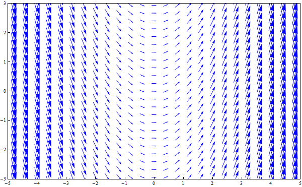
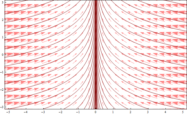
 Next we find the flow of this vector field:
\begin{equation*}
f'(t) = -f(t) \qquad \text{and} \qquad g'(t) = 1.
\end{equation*}
The solutions are
\begin{equation*}
x = f(t) = c_1 \exp(-t) \qquad \text{and} \qquad y = g(t) = t + c_2.
\end{equation*}
Or, eliminating $t$ we have $x = c \, \exp(-y)$ where $c$ is an arbitrary constant.
Next we find the flow of this vector field:
\begin{equation*}
f'(t) = -f(t) \qquad \text{and} \qquad g'(t) = 1.
\end{equation*}
The solutions are
\begin{equation*}
x = f(t) = c_1 \exp(-t) \qquad \text{and} \qquad y = g(t) = t + c_2.
\end{equation*}
Or, eliminating $t$ we have $x = c \, \exp(-y)$ where $c$ is an arbitrary constant.
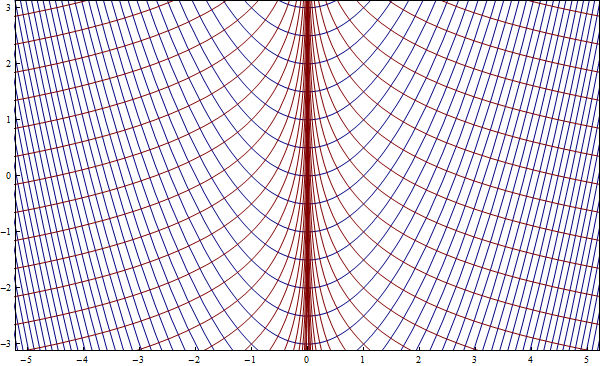
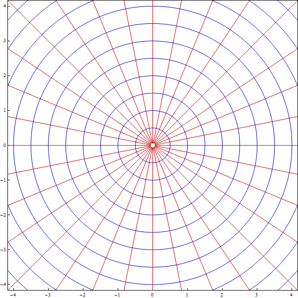
 In this way we have obtained two families of mutually orthogonal curves:
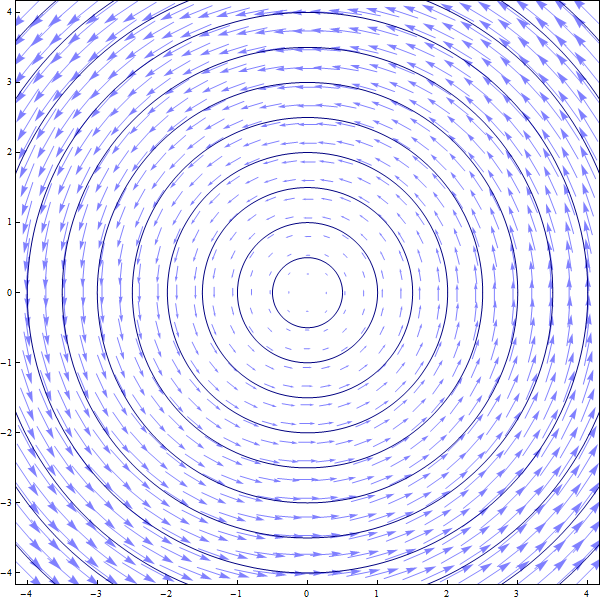
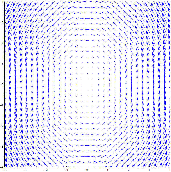
 To get the explicit solutions for the flow lines we have to find the parametric curve $x=f(t), y=g(t),$ by solving the differential equations
\begin{equation*}
f'(t) = -g(t) \qquad \text{and} \qquad g'(t) = f(t).
\end{equation*}
The solutions are
\begin{equation*}
x = f(t) = r \cos(t) \qquad \text{and} \qquad y = g(t) = r \sin(t)
\end{equation*}
where $r$ is an arbitrary positive constant. Or, eliminating $t$ we have $x^2 + y^2 = r$ where $r$ is an arbitrary positive constant.
To get the explicit solutions for the flow lines we have to find the parametric curve $x=f(t), y=g(t),$ by solving the differential equations
\begin{equation*}
f'(t) = -g(t) \qquad \text{and} \qquad g'(t) = f(t).
\end{equation*}
The solutions are
\begin{equation*}
x = f(t) = r \cos(t) \qquad \text{and} \qquad y = g(t) = r \sin(t)
\end{equation*}
where $r$ is an arbitrary positive constant. Or, eliminating $t$ we have $x^2 + y^2 = r$ where $r$ is an arbitrary positive constant.
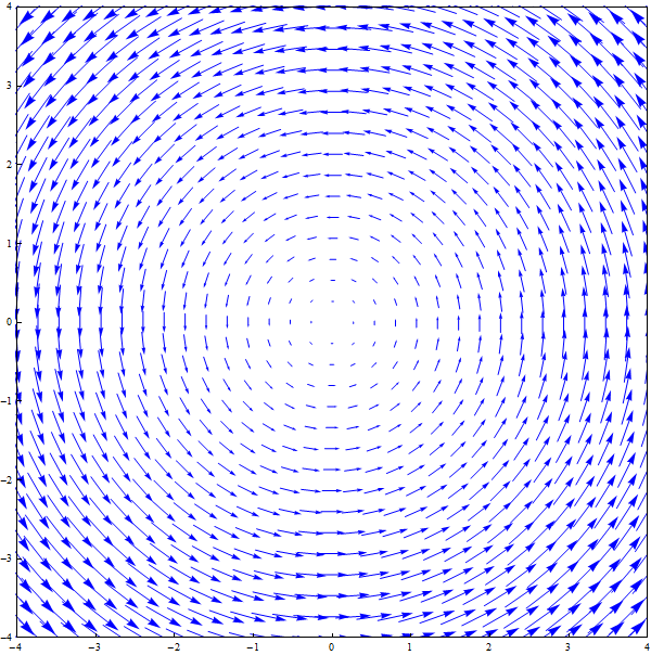
 The orthogonal vector field to $\vec{F}$ is
\begin{equation*}
\vec{G}(x,y) = (-x) \vec{\imath} + (-y) \vec{\jmath}
\end{equation*}
The orthogonal vector field to $\vec{F}$ is
\begin{equation*}
\vec{G}(x,y) = (-x) \vec{\imath} + (-y) \vec{\jmath}
\end{equation*}
 Next we find the flow of this vector field:
\begin{equation*}
f'(t) = -f(t) \qquad \text{and} \qquad g'(t) = -g(t).
\end{equation*}
The solutions are
\begin{equation*}
x = f(t) = c_1 \exp(-t) \qquad \text{and} \qquad y = g(t) = c_2 \exp(-t).
\end{equation*}
Or, eliminating $t$ we have $y = c \, x$ where $c$ is an arbitrary constant.
Next we find the flow of this vector field:
\begin{equation*}
f'(t) = -f(t) \qquad \text{and} \qquad g'(t) = -g(t).
\end{equation*}
The solutions are
\begin{equation*}
x = f(t) = c_1 \exp(-t) \qquad \text{and} \qquad y = g(t) = c_2 \exp(-t).
\end{equation*}
Or, eliminating $t$ we have $y = c \, x$ where $c$ is an arbitrary constant.
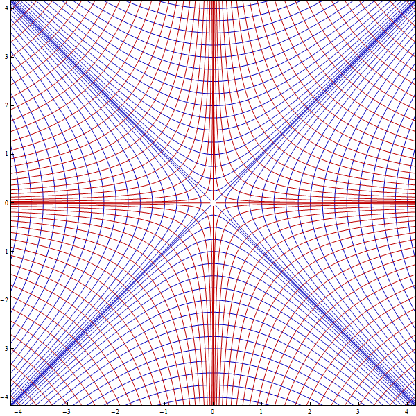
 In this way we have obtained two families of mutually orthogonal curves:
 To get the explicit solutions for the flow lines we have to find the parametric curve $x=f(t), y=g(t),$ by solving the differential equations
\begin{equation*}
f'(t) = g(t) \qquad \text{and} \qquad g'(t) = f(t).
\end{equation*}
The solutions are
\begin{equation*}
x = f(t) = r \cosh(t) \qquad \text{and} \qquad y = g(t) = r \sinh(t)
\end{equation*}
where $r$ is an arbitrary constant. Or, eliminating $t$ we have $x^2 - y^2 = c$ where $c$ is an arbitrary constant.
To get the explicit solutions for the flow lines we have to find the parametric curve $x=f(t), y=g(t),$ by solving the differential equations
\begin{equation*}
f'(t) = g(t) \qquad \text{and} \qquad g'(t) = f(t).
\end{equation*}
The solutions are
\begin{equation*}
x = f(t) = r \cosh(t) \qquad \text{and} \qquad y = g(t) = r \sinh(t)
\end{equation*}
where $r$ is an arbitrary constant. Or, eliminating $t$ we have $x^2 - y^2 = c$ where $c$ is an arbitrary constant.
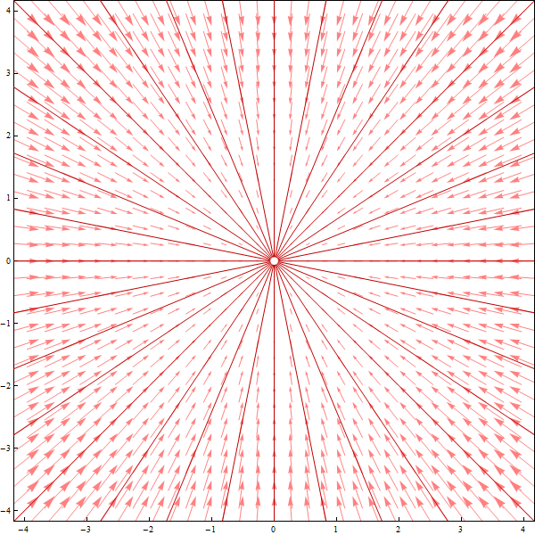
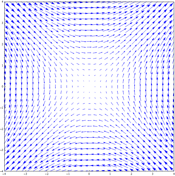
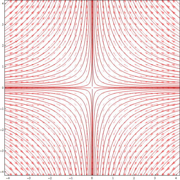
 The orthogonal vector field to $\vec{F}$ is
\begin{equation*}
\vec{G}(x,y) = (-x) \vec{\imath} + y \vec{\jmath}
\end{equation*}
The orthogonal vector field to $\vec{F}$ is
\begin{equation*}
\vec{G}(x,y) = (-x) \vec{\imath} + y \vec{\jmath}
\end{equation*}
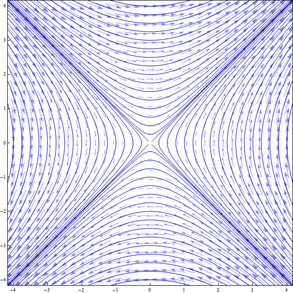
 Next we find the flow of this vector field:
\begin{equation*}
f'(t) = -f(t) \qquad \text{and} \qquad g'(t) = g(t).
\end{equation*}
The solutions are
\begin{equation*}
x = f(t) = c_1 \exp(-t) \qquad \text{and} \qquad y = g(t) = c_2 \exp(t).
\end{equation*}
Or, eliminating $t$ we have $xy = c$ where $c$ is an arbitrary constant.
Next we find the flow of this vector field:
\begin{equation*}
f'(t) = -f(t) \qquad \text{and} \qquad g'(t) = g(t).
\end{equation*}
The solutions are
\begin{equation*}
x = f(t) = c_1 \exp(-t) \qquad \text{and} \qquad y = g(t) = c_2 \exp(t).
\end{equation*}
Or, eliminating $t$ we have $xy = c$ where $c$ is an arbitrary constant.
 In this way we have obtained two families of mutually orthogonal curves:
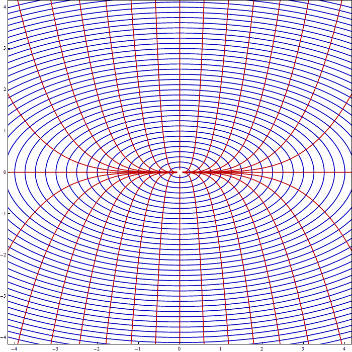
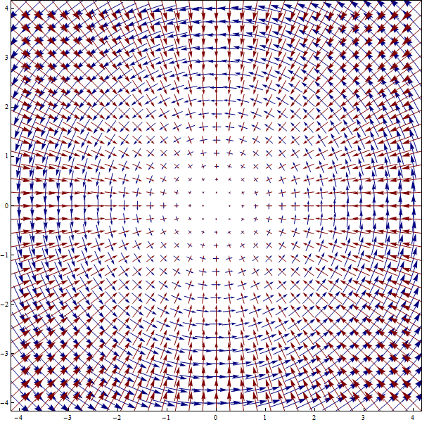
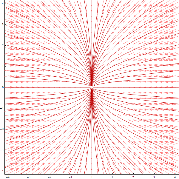
 To get the explicit solutions for the flow lines we have to find the parametric curve $x=f(t), y=g(t),$ by solving the differential equations
\begin{equation*}
f'(t) = -g(t) \qquad \text{and} \qquad g'(t) = 2f(t).
\end{equation*}
Solutions are
\begin{equation*}
x = f(t) = r \cos\bigl(\sqrt{2}t\bigr) \qquad \text{and} \qquad y = g(t) = r \sqrt{2} \sin\bigl(\sqrt{2}t\bigr)
\end{equation*}
where $r$ is an arbitrary positive constant. Or, eliminating $t$ we have $x^2 + \frac{y^2}{2} = r$ where $r$ is an arbitrary positive constant.
To get the explicit solutions for the flow lines we have to find the parametric curve $x=f(t), y=g(t),$ by solving the differential equations
\begin{equation*}
f'(t) = -g(t) \qquad \text{and} \qquad g'(t) = 2f(t).
\end{equation*}
Solutions are
\begin{equation*}
x = f(t) = r \cos\bigl(\sqrt{2}t\bigr) \qquad \text{and} \qquad y = g(t) = r \sqrt{2} \sin\bigl(\sqrt{2}t\bigr)
\end{equation*}
where $r$ is an arbitrary positive constant. Or, eliminating $t$ we have $x^2 + \frac{y^2}{2} = r$ where $r$ is an arbitrary positive constant.
 The orthogonal vector field to $\vec{F}$ is
\begin{equation*}
\vec{G}(x,y) = (-2x) \vec{\imath} + (-y) \vec{\jmath}
\end{equation*}
The orthogonal vector field to $\vec{F}$ is
\begin{equation*}
\vec{G}(x,y) = (-2x) \vec{\imath} + (-y) \vec{\jmath}
\end{equation*}
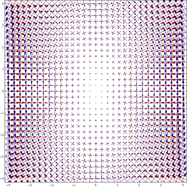 Next we find the flow of this vector field:
\begin{equation*}
f'(t) = -2f(t) \qquad \text{and} \qquad g'(t) = -g(t).
\end{equation*}
The solutions are
\begin{equation*}
x = f(t) = c_1 \exp(-2t) \qquad \text{and} \qquad y = g(t) = c_2 \exp(-t).
\end{equation*}
Or, eliminating $t$ we have $x = c y^2$ where $c$ is an arbitrary constant.
Next we find the flow of this vector field:
\begin{equation*}
f'(t) = -2f(t) \qquad \text{and} \qquad g'(t) = -g(t).
\end{equation*}
The solutions are
\begin{equation*}
x = f(t) = c_1 \exp(-2t) \qquad \text{and} \qquad y = g(t) = c_2 \exp(-t).
\end{equation*}
Or, eliminating $t$ we have $x = c y^2$ where $c$ is an arbitrary constant.
 In this way we have obtained two families of mutually orthogonal curves:
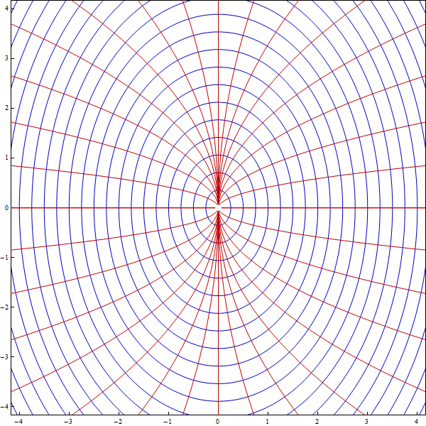 Here we encountered the family of ellipses with the ratio of vertical and horizontal axis being $\sqrt{2}$. There is nothing exceptional about this family. So, the above picture suggests an animation of a collection of families of ellipses with the ratios of vertical and horizontal axis being between $1/2$ and $2$, each family accompanied by its orthogonal family of curves.
Place the cursor over the image to start the animation.