ESCI497Z: UAS for Environmental Research and Monitoring

Post Point Heron Colony Survey; Introduction to Agisoft Metashape

Updated 10/10/2022

Objective: We will be using imagery acquired using our 3DR Solo to survey the Great Blue Heron colony at near Post Point. As you may know, each year about 10-20 Great Blue Herons nest near Post Point. The colony is not active during the fall (October) but we’ll see if UAS provide a viable method for locating nests. This exercise will familiarize you with the use of Agisoft Metashape (AM) software. Note that the older version of this software was called Agisoft Photoscan so at times in this document I may screw up and refer to Photoscan when I’m really talking about Metashape. And, at times we will be using documentation from the old Photoscan software since they have not released an updated tutorial for Metashape. Metashape has some improvements and the interface is a bit different than Photoscan. Anyway, the AM software will enable us to create an orthomosaic from all of our images and it will also enable us to create a Digital Surface Model from this imagery. AM is comparable to Pix4D, Drone Deploy and Drone2Map, an ESRI product that just came out but I’ve not yet had a chance to use. All of these are “Structure from Motion” (SFM) software packages and not sure, but it think they may all be using algorithms purchased/licensed from Agisoft.

PROCEDURES:

Step 1: Get the data. Go to J:/Saldata/ESCI-497/post_pt_heron. Copy the entire post_pt_heron folder and then go to C:/temp on our computer, create a folder with your name and paste the post_pt_heron folder there. So, you should now have a folder on your computer called C:/temp/yourname/post_pt_heron that contains everything from the post_pt_heron folder on the J-drive.

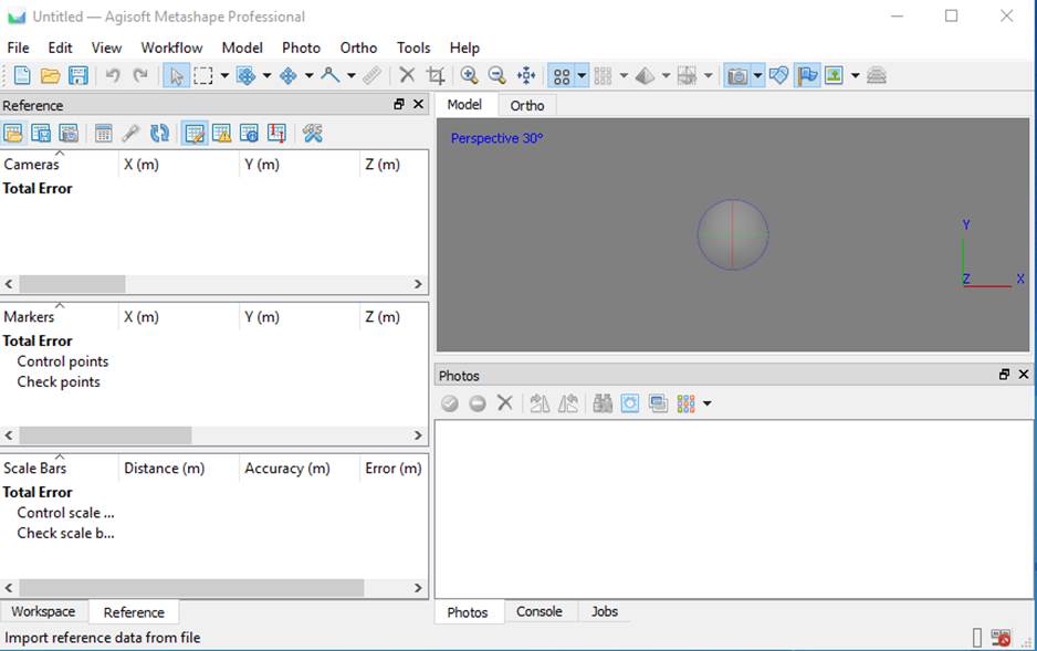
Step 2: Open Agisoft. Graze through the vast maze of software on your computer and find Agisoft Metashape and open it. This will bring up a screen that looks like this.

In the lower left corner of this window, click on the References tab to bring up this:

MAlso, go the Post_pt_heron folder and open the PS_1.3-Tutorial (BL)-Ortho, DEM (with GCPs).pdf file. We will be following this tutorial (mostly) but I’ll add a few comments/clarifications as we work through it. As noted above, this is a tutorial for the older Agisoft Photoscan software and interface for Metashape is a bit different. I’ll try to walk you through the differences.

Set Phtoscan Preferences: You can skip the stuff in this section. Defaults should be fine.

Step 2 Add Photos

Our Post_pt_heron folder includes a subfolder called /120mflt. This includes about 75 images acquired on a programed flight over the study area at an elevation of 120m (~400 feet). Here is an overview of the area covered by the imagery:

OK, now follow the tutorial instructions to Add Photos. When you do so, you will note that all of the images appear in the Photos section (lower right) of the AM screen and a list of all of the image names appear in the Cameras section (upper left). Unfortunately, the GPS in my camera wasn’t working when I did this flight so there are no X, Y Z positions for the cameras. If the images had included geotagged, this information would appear in the Cameras section along with the image names. In some cases, you might have geotags for the images in a separate file and you could load these following the instructions. If you do have geotags for your images, a bunch of blue dots would appear in the grey Model window showing the relative position of each image.

But we can move forward without this information……so just skip all of the Load Camera Positions instructions.

Step 3: Camera calibration

All cameras and lens have distortion to some degree. You can use an auxiliary program, appropriately called “LENS” to gather a bunch of obscure parameters to characterize your particular camera. I will not pretend that I understand what much of this but getting this info for your camera improves the quality of your results. It is pretty straightforward. Using the LENS software, you display a checkerboard pattern on your computer screen, take a few photos with your camera, load the photos into the software, push a few buttons and, SHAZAM, you get a camera calibration file.

You can proceed WITHOUT a camera calibration file. Without one, the software will derive one using the imagery but you get a better result if you have one.

So, follow the tutorial instructions to load the camera calibration file (wwucolor2.xml). Click on the folder icon to load this file.

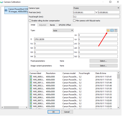
Note that the interface in Metashape is a bit different than the Photoscan interface shown in the tutorial. After loading the hit OK to close the Camera Calibration dialog box.

Note that, you should deviate from the tutorial just a bit in that YOU SHOULD NOT check the Fix Calibration flag!!! Leaving this unchecked will yield a much better georegistration result below.

Step 4: Align Photos

This is the first really time consuming step. In the Align Photos dialog, set the Accuracy to Medium and make sure that Generic preselection is checked. You would use Reference preselection if your images were geotagged and this would help speed up the alignment process since the software would have a rough idea of which photos were near each other. With Generic preselection, the alignment process takes longer since the software doesn’t have this information. Click on the Advanced pull down to see more options.

Key points are locations in an image where there is some variability. These represent unique features in each image which could be useful in matching up photos. You want as many as possible in each image but setting this too high can result in a large number of unreliable points. Go with 60,000.

Tie points are key points that match across multiple images. Using a value of 0 does not set an upper limit (which seems rather backwards I know) so go with a value of 0

Click on OK to begin the alignment process. This should take about 5 minutes to run.

Be patient. Recognize that the software is looking for “tie points” – obvious features – on every image and looking for matches on every OTHER image in the dataset. This involves bazillions of calculations and comparisons to align all of the images.

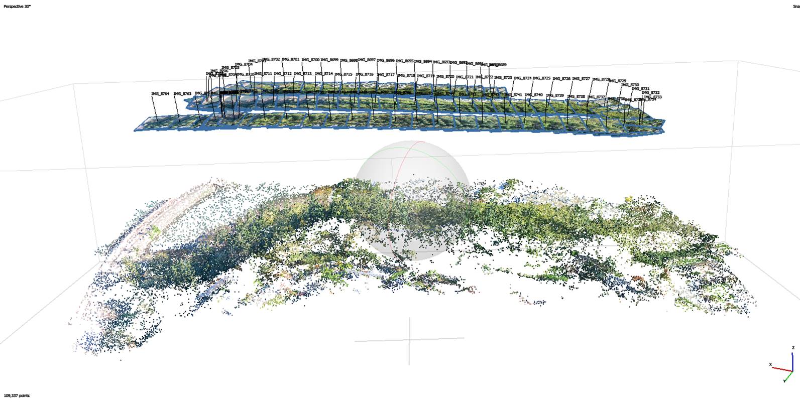
When it finishes running, you will see something like this in the Model window. This is what is known as a “sparse point cloud.”

You may need to resize all the sub-windows to see this. And, if you click in the Model window, you can use your mouse roller to resize the image.

If you do not see this, don’t panic. It’s time to learn a few tricks

Toggle camera locations on/off:To make the blue squares appear (or disappear), click on the camera icon on the toolbar at the top of your screen. Each thumbnail represents the approximate footprint of an image.

Image rotation: Also note the rather ghostly sphere in the center of the image and the little X, Y, Z axis in the lower right. You can rotate the image in 3 dimensions by placing your cursor in the screen somewhere, push and hold the left mouse button, and drag your mouse around. Note that your image might be UPSIDE DOWN when it first appears. By that I mean that you may be viewing your image from underground. Weird, I know

Try to get a somewhat side view of your image. With the thumbnails on you should see something like this:

The small black line indicates the position the camera was pointing (usually straight down but sometimes at a slight angle).

Zooming: Use the roller button on your mouse to zoom in or out. Note that as you zoom in, you will see the individual names appear. These disappear as you zoom out.

Moving the image: When zoomed in, you may want to examine a different part of the image. To move around, push and hold the right mouse button, and drag your mouse around.

Sparse Point Cloud: OK with the thumbnails turned off, what ARE those green and white and blue dots in your image? While aligning the images, AM created what is known as a sparse point cloud. This consists of a modest number of points (in this case only 109,337 points) each with an X, Y, Z coordinate and a color derived from the photos. A bit later, we’ll create a dense point cloud with millions of points that will provide us with a much better 3-dimensional representation of our study area.

Before we can do this, we need to locate some ground control points (GCPs) in our images. AM refers to GCPs as Markers.

Step 5: Place Markers

SAVE YOUR WORK SO FAR!

To save your work thus far, go to File-Save As and give your project a file name. This will create a file with a .psx suffix. If you wanted to quit at this point, you could come back and open this .psx file and you would come right back to where you left off. You should get in the habit of saving your work periodically as you move through this project. Note added 4/24/2020: If you take a look at the file size for your *.psx file, you will note that it is quite small, perhaps 1 Kb or so. This file is nothing more than a bunch of pointers to a bunch of larger files. All of these larger files are contained in a folder with the same name as your *.psx file. This means that at the end of a work session, when you move your files from your workspace in C:/temp/yourfoldername you should be sure to move note just the *.psx file but also the folder with the same name.

Step 6: Place Markers

Ideally, I would go out to the site before flying with a VERY good GPS unit and, log X, Y, Z coordinates for 10-12 locations and mark these locations in a way that would be very visible in the photos. You saw some of this at the Glacier Springs site. Ideally, I’d like these coordinates to be accurate to within a few centimeters. Obtaining this level of accuracy requires a GPS unit that costs several thousand dollars. Your $300 Garmin only accurate to within about 3-5 m. You need centimeter accuracy if you want to be able to line up imagery from different dates to carry out change detection.

A quick and dirty approach: If you do not need to line up imagery with high precision, one quick and dirty approach is to just use Google Earth. Zoom in on the imagery, find a prominent feature and record the coordinates from Google Earth (latitude, longitude and elevation). This will probably get you to within a meter or two and this will be good enough for our current effort.

So, start this process by following the tutorial instructions to Build Mesh. But in the Build Mesh dialog, be sure to set the Source data to Depth maps and be sure to set the Quality and Face count to Low to reduce processing time.

Click OK to run this. This just takes a few minutes and will create something like this:

You can get back to your sparse point cloud image by clicking on the icon on the top toolbar.

I have coordinates for five GCPs that we can use for our study area. More would be better but this will be sufficient for our purposes here. The first two are on the south side of our study area on residential streets. (Note that I DID NOT fly over this residential area but the field of view of the camera was such that I did get a bit of coverage of a handful of houses). Here are the rough positions of the first two GCPs (this is an image from Bing, not my UAS imagery).

Starting with GCP#1, go to AM and zoom in a bit on this part of your image. Make sure that you have the camera locations turned on. Zoom in enough so you can see the image labels. Make a guess regarding which image might include this GCP.

I’m guessing that this GCP might be visible down near the turn at the SE corner of the study area.

So, this looks like it might be image #8734. Down in the Photo section of the screen, scroll down to find this image. When you do, double-click on it. This will bring up a second tab in the upper right section of the screen that will display this image. Like this:

Note that you will now see two tabs in the upper right screen, one for the Model (the thing that you were viewing before) and one showing image #8734. And, GCP#1 is right in the middle of this cul-de-sac.

So, follow the tutorial instructions to place your first “Marker” right dead center in this cul-de-sak. You can use the roller button on your mouse to zoom in on the image. And you can left-click and hold to move around in the image. So, here is my first marker:

Yes! I know that the marker placement feels a bit arbitrary in this case but you can probably get in placed within ~0.5 m or so of the center. If you need to adjust the placement a bit, put the cursor on the marker, left-click and hold and drag it a bit.

OK, so you have located Marker 1 on a single image. Now we need to locate it on every other image where it is visible. Start by looking at the next image. In the Photo section of the screen, double-click on image #8735. You will note that there is a blue flag in the cul-de-sac. AM has made a guess as to where Mark 1 is probably located in this image. You should zoom in and check it. You may decide to drag it just a bit….or not. But you should click on the marker even if you choose not to move it. When you do, the flag will change to green indicating your confirmation of this position.

Now you need to check ALL the other images where this marker if visible. AM can narrow your search. On the middle left of the screen, you will see a panel that says Markers and point 1. Right-click on point 1 and you will see an option to filter photos by markers. Select this and you will now see that there are only seven image in the Photos panel. Click through each of these images and confirm the marker location in each one.

After doing so, click on the icon in the Photos panel to go back to viewing all of the images.

Find GCP#2

Click on the Model tab in the upper right panel so you can see the entire study area. Make a guess on the location of GCP#2. Try image #8747. This is a tough one since there are quite a few trees. Here is the location for this one:

As for Marker 1, find this spot in the next image, then filter photos by marker. This yields about 17 images that potentially include this marker. However, the trees will block your view of the road surface in some cases, like this one:

In this case, you should right-click on the point and select Remove marker. Doing so will remove the blue flag and replace it with a funny looking grey thingy.

Continue checking all of the other photos for Marker 2.

GCP#3-5

Here are the general locations for the remaining GCPs

OK, now add markers for each of these 3 points. Points 3 & 5 are dead center in these trail intersections. Point 4 is the northeast corner of that white square. This is an example of a really really good choice for a GCP in that the exact location of the GCP is very obvious in the imagery. Admittedly, correctly locating the other 4 GCPs in this exercise is somewhat subjective. But again, this is good enough for our purposes here.

AGAIN, SAVE YOUR WORK SO FAR!

To save your work thus far, go to File-Save. As indicated above, this will create a file with a .psx suffix. If you wanted to quit at this point, you could come back and open this .psx file and you would come right back to where you left off. You should get in the habit of saving your work periodically as you move through this project.

Input Marker Coordinates

Follow the tutorial instructions to Input Marker Coordinates ( on the Reference pane) using the file post_pot5gcp.txt. Use these settings:

Note that you need to specify the coordinate system that you are using (WGS84 in our case) and make sure that you specify the correct columns for each parameter and the starting row number, then click OK.

In the middle left panel, use the slider to see the Error associated with each marker. At this point, it will just show the error in terms of # of pixels; probably around 2 pixels for each one. Not great but OK for now.

Optimize Camera Alignment

Carefully follow the tutorial instructions here. Use these settings:

As indicated in the instruction, be sure to uncheck all of the images and check all of the markers, then go to Tools-Optimize camera alignment and use:

When complete, take a look at the Error for each of your markers. Now much better. Mine range from 0.03-0.13 m for mine. Yours will be a bit different depending on how carefully you placed your markers.

AGAIN, SAVE YOUR WORK SO FAR!

Set the Bounding Box

Create Dense Point Cloud

This is by far the most time consuming step. I’d go with these options:

With this dataset, it may take 15 minutes or so, maybe a bit more. I’ve had projects with 3-4000 images that I run overnight on my computer. If you take a look at the performance tab on your Task Manager, you will note that the CPU is maxed out during this operation. This is a good time to take a break.

Mission Planner: While this is running, we may spend some time providing a brief intro to the use of Mission Planner.

After this step completes…….

Let’s take a look at the dense point cloud. To do so, click on the dense point cloud button along the top of the screen. This should result in a display like this:

This is analogous to a First Return LIDAR surface. Note that this dense point cloud consists of over 7 million points. Pretty cool isn’t it!

Drape the image over the point cloud: click on this button to get:

And moving on…..

Build Mesh: Do this.

Edit Geometry: SKIP THIS STEP

Build Texture: SKIP THIS STEP

Build DEM: Do this. Very fast. It will looks something like this:

Build Orthomosaic: Do this. A few minutes. It will look something like this:

The ortho will be a cleaner image than the image draped over the dense point cloud.

Herons? And what about those heron nests?

Following the instructions in the tutorial, take a look at the ortho image. Zoom in on the area of deciduous trees just to the west of point 4 and south of the big round thing with the spokes at the sewage treatment plant. See this:

The arrows point to a couple of Great Blue Heron nests. Look around and see how many you can see.

Export Orthomosaic: Do this. And note that, at this step (and for the DEM as well), if you’d like, you can choose to export the Ortho in a projection other than the one that you have used thus far. So, if your ultimate goal is to use this product with some other GIS layers, you may want to export the ortho in the same projection as your other layers. At the same time, you can choose to alter the pixel size somewhat. For example, in this case, we’ve been working in WGS84 with our X and Y coordinates in degrees. So the default pixel size will also be in degrees. Like this:

Instead, you might choose to export this using a UTM projection or State Plane with the pixel size in meters or feet. And, if you do choose to go with UTM, for example, you will note that the default pixel size is a bit goofy; not a nice round number. So you might choose to round it off to something simple. Perhaps 0.04 m or 0.03 m rather than 0.0331902 m.

Export DEM: Do this. Note that, as a rule of thumb, the pixel size for the DEM will, by default, be about 4X the pixel size of the ortho.

If you’d like, you can bring the tiffs for both your DEM and your ortho into Arc to play with them a bit more. This is optional.

Generate Report:

This is not mentioned in the tutorial but I feel this is a nice thing to do. Similar to what you did in exporting the Ortho and the DEM, go to File-Generate Report , then select a file name. This generates a nice PDF file with all sorts of geeky stats on your project.

AGAIN, SAVE YOUR WORK!

Lab Report: OK I’d like you to write a brief lab report based on your work. On the Lab Exercises Index page, there is a link to a Lab Report Guide that explains the format that I would like you to use for your report. Your report will be due on April 27 at 1:00PM.

Note added 10/112022: What should go in your lab report? The motivation for this flight was to see if we could use the UAS imagery to inventory (count) the Great Blue Heron nests. I’d say the answer to this is yes. So in your results, tell me how many nests you can find. Also note that the study area includes both conifers and hardwoods. What is the range of heights that you find in the area with the hardwoods and what is the range of heights for the conifers. You can get this by simply using your cursor to sample 10-20 trees in each area and give me the range. And give me these heights relative to the takeoff location which is at marker location #3. You should also report your spatial resolution; the pixel size. This is in the report that we generated from Agisoft. You might include some screenshots from this report. What was the Error for your markers? How was the coverage in terms of # pictures covering various parts of the study area? In your discussion, you should also discuss what could be done to obtain better coverage of the study area? Maybe fly lower for higher spatial resolution. But what are the limits to doing this (height of tallest trees). Does the flight plan provide adequate coverage of the area or does it need to be bigger? What about our markers (Ground Control Points)? Did we have enough? Were they well marked in the field and easy to precisely locate in the images? Did we have accurate coordinates for these GCPs?