January 2018

Goals for the new year: answer some seal questions

MacKenna Newmarch, undergraduate student

1 January 2018

This month I began to examine our behavioral data to improve my research question and narrow my interests.  From previous years, we have been able to assign approximately 3,000 surfacing events to individual seals from 2011 through 2015.  These data tell us where in the creek seals were located, how long they surfaced for, the behavioral state that they are displaying, and whether they caught a fish or not.  I chose to examine the relationship between how many days a seal showed up at the creek and the number of times they caught a fish, which can give us clues about individual differences in foraging behavior.  If there is a significant relationship between number of visits and fish caught (my definition of foraging success), one can infer little individual differences given that the foraging success rate would mostly depends on how often a seal visits the creek.  On the other hand, a lack of relationship would suggest that success rate is not dependent on the number of visits and that other factors (such as type of hunting behavior) play an important role.

I organized our surfacing data into dates in which a particular seal visited the creek and totaled the number of fish that we observed being caught by that individual.  To examine the relationship between number of visits and foraging success, I displayed the data graphically using a scatterplot.

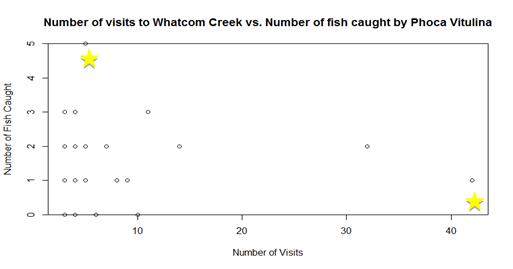
Figure 1. Number of fish caught relative to number of seal visits to Whatcom Creek.

The data in the figure above suggests that there was no relationship between the number of fish caught and the number of times a seal visited the creek.  As seen by the points starred, a seal can rarely show up but catch a fish every time, or show up frequently but rarely catch a fish.  This initial exploration suggests that there are other variables besides visiting the creek affecting the success of seals in catching fish.  I will then look further into which factors affect foraging success and how success varies on an individual basis.

The first step is to distinguish between actively hunting salmon at the creek versus merely stopping for a visit.  To that end, I have defined five behavioral states indicative of active hunting: 1) turned upside down for a better view under the surface, 2) surfacing/scanning on the creek bank, 3) large, noticeable wake, 4) jumping out of the water, and 5) consistent surfacing (more than half of the time in the creek) in the upper creek/stairs eddy region.  The two locations chosen to define active hunting (upper creek and stairs eddy) are important because salmon are funneled into the fish ladder at the stairs eddy or continue to swim upstream into a small cove.

One factor that I will examine as potentially affecting the foraging success of seals is the location where hunting occurs.  I will be splitting the creek into six sections to describe the locations of various behaviors.  Vertically, the creek will be split into the middle and the banks.  This is necessary if I am to compare behavior on the banks where hunting occurs with higher frequency versus the middle.

Defining these regions will be interesting as it can allow me to find “hot spots” for particular individuals.  We may see most seals hunting in region 4 but seal 12 might have significantly higher success in region 2.  The regions for this variation can be analyzed and may allow us to discover traits that increases success in hunting.  This could be important ecologically if we find, for example, that the presence of rocky substrate in this region is likely what contributes to a harbor seals success.  This could also be a method to discover how best to implement endangered salmon conservation and protect them from harbor seals so their populations are allowed to flourish.  If we know exactly what is allowing particular harbor seals to hunt at a success rate 5x higher than others, we can decide how best to keep them from doing so.

Before I will be able to analyze these specifics, much of our behavioral data from 2015 needs to be updated.  Some photos of seals that we had previously identified and subsequently tied to specific behavioral events turned out to be incorrect.  I would also like to include data from 2016 which requires identifying several other photos and tying them to surfacing events.  I have lots of work ahead of me in the new year before I am allowed any rewarding discovery.

Cannot wait to see what the future holds for our project!

Questions for surveys

Alisa Aist, undergraduate student
1 January 2018

As I am creating my survey questions I have noticed in several scientific papers that people use many different types of questions, the most common of which are open-ended and Likert-type.  Each type of question will result in certain types of answers.  In order to get the answers you want, one has to carefully consider the type of questions to ask.

There are eight types of survey questions, each with their own pros and cons.  There are closed-ended questions, which are best defined as questions that offer answers for the respondent to choose from.  The ways these answers are formatted can be very different and will determine the information one gets.

Rating-scale questions can be useful close-ended questions where the options can be formatted Likert-type or as a semantic differential.  A Likert-type rating scale is one where the respondent is asked whether they agree or disagree with a statement, often there are multiple levels for the respondent to agree or disagree with and a neutral option as well.  These questions are very flexible and are easy to compile and analyze, however, the respondent does not state the reason for the answer.  Semantic differential is a scale where one side is an extreme and the other is the other extreme, such as 1 representing short and 10 representing long.

Another kind of closed-ended question is the classic multiple-choice question.  It is easy to answer, but respondents have a limited number of answers and do not always have an opportunity to answer how they want.  There are also rank-order questions in which people rank answers based on importance, allowing the researcher to define the “best” and “worst” answers, but without knowing why.  Dichotomous questions have only two answers, such as yes/no questions, which prevents ambiguity but there is no elaboration.

There are also open-ended questions, which allow respondents to express their opinions to their fullest extent and emphasize what they want.  On the other side, they can take a long time to collect and analyze, and it is also possible to ask leading questions which can skew the results.  One way that researchers use to analyze open-ended questions is to look for keywords that indicate one opinion vs. another.

It is very important for a researcher to carefully consider how much time they will get with each interview and how much time they have to analyze the results.  The type of questions are just one aspect an interviewer has to consider before starting.

Sex and specialization

Madelyn Voelker, graduate student

11 January 2018

One interesting factor I am considering in my thesis is the effect of sex on the level of specialization. A fun way to investigate this question is through graphical representations of the averages and confidence intervals of specialization values. This allows you to observe patterns in the data. In the graphs below the average is denoted by a dot and the 95% confidence interval is indicated by the spread of bars on either side of the average. The y axes indicate the level of specialization, which is measured in psi. A psi value of one indicates a total generalist, a psi value of zero indicates a total specialist. The x axes show during which month each set of scats were collected. The scat where also separated by sex, which is denoted in the graphs as well.

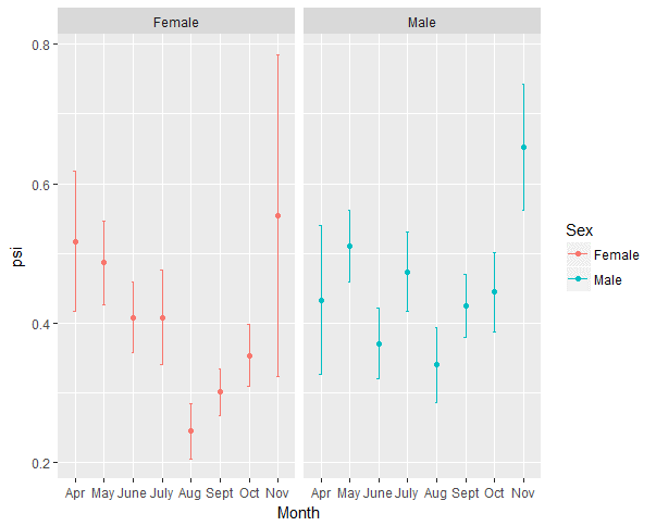
Figure 1. Average psi values across four haul-outs (Belle Chain, Cowichan Bay, Comox, Fraser River) during 2012 and 2013. The left graph shows females, the right graph shows males.

A very interesting pattern that this graph suggests is that female seals have a dip in their psi values during July and August. The same dip is not present in males. This suggests that during the months of July and August females change their feeding behavior in a different way than male seals. Specifically, females are becoming more specialized during those months relative to the spring and fall months. One potential cause for this different pattern in each sex would be the act of giving birth, which happens at these haul-outs in July and August.

One issue with this type of analysis is it does not account for the unbalanced nature of the data set. This data set is somewhat unbalanced because certain haul-outs had more scat collected at than others. This means that the averages represented on the graphs are influenced more by certain locations than others. Thus, it is important to look at the patterns within each haul-out site. The following figures break up the collected scat by haul-out and sex. An additional haul-out, Baby Island, was included in Figure 2 and 3. Baby Island was not included in Figure 1 because collections only occurred there in 2016. An additional year (2014) of collections at Cowichan Bay was also included. The same pattern observed above in females is reflected at Belle Chain, Cowichan Bay, and Comox (Figure 2). However, the pattern is less district in all cases. Additionally, male seals again lack a drop in psi centered around July and August (Figure 3). Thus, it seems like the overall pattern present in the combined data set is true in at least some locations, but perhaps not all.

While none of the analysis presented here are conclusive, they definitely point to some interesting phenomena. As mentioned in my previous blog, I am also approaching these questions using modeling. Hopefully the combination of multiple data analysis approaches will allow me to paint a fairly clear picture of the different factors influencing specialization.

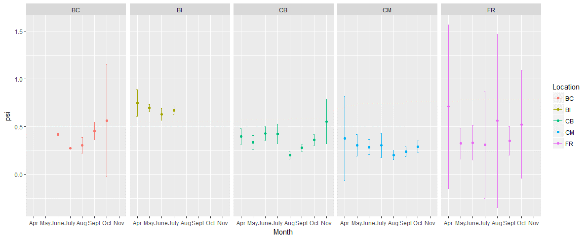
Figure 2. Average psi values and 95% confidence intervals for all female scat collected within each month at each site.
BC = Belle Chain, BI = Baby Island, CB = Cowichan Bay, CM = Comox, FR = Fraser River.

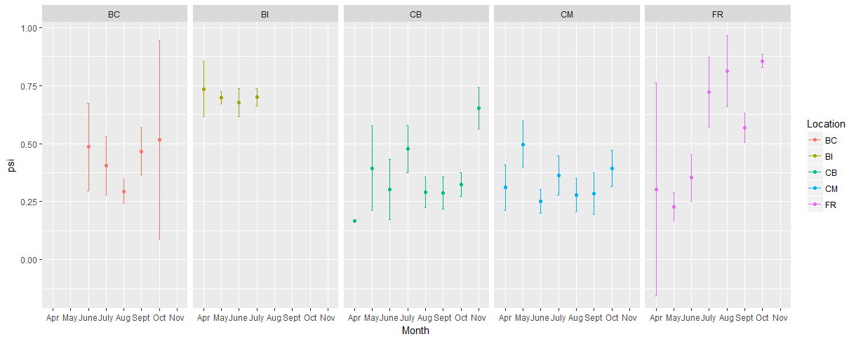
Figure 3. Average psi values and 95% confidence intervals for all male scat collected within each month at each site.
BC = Belle Chain, BI = Baby Island, CB = Cowichan Bay, CM = Comox, FR = Fraser River.