JANUARY 2020
Grace's Blog
Grace Freeman, graduate student
1 January 2020
This year Santa brought me a hand surgery for Christmas, so please excuse the brevity of this blog post. I’m grateful I don’t have classes right now as writing left-handed and typing one-handed is difficult to say the least!
I’ve been back home in Minnesota for about a week, and I’m appreciative for a break from classes and TAing - even if it comes with a foot of snow! The end of the quarter was crazy as promised, but this time away has given me a chance to get caught up on proposal writing and paper reading. I also downloaded some preliminary data before leaving the lab for break, so it’s been fun to dive into some statistical analyses to see exactly what trends I may find and questions I may be able to answer. I’m feeling ready to hit the ground running when I return to Bellingham this week and start finalizing my proposal and research plan. Stay tuned for more on that in January!
Blog Post 4
Bobbie Buzzell, graduate student
1 January 2020
Winter break quickly came and is even more quickly coming to a close, but a lot of great things have happened since the beginning of December. Back in October, I applied for a small travel grant through Western’s Research Sponsored Programs (RSP). This grant would fund my stay in Seattle where I would receive introductory training in fish bone identification with William “Bill” Walker, a food habits specialist contracted with NOAA (see blog post 2). I received notice of approved funding just before my planned training dates. Timing couldn’t have been better!
When I began training with Bill in mid-December, we started with the basics. I would need to take the time to learn and memorize bones from the entire fish skeleton. There was really no other way around it. He reviewed the bones with me that are the most useful in identifying exact species of fish. While most of the bones might be considered “junk” (as Bill would put it), there are a select number of bones that provide the most information, such as otoliths (ear bones), maxillas, dentaries, and articulars (portions of the jaw).
We sifted through several of my samples while I was training with Bill. I learned characteristic features for a couple of the commonly found fish species in my scats so far: the stellate scales from irish lords, and the preopercle spine from staghorn sculpins. As he walked me through each of the bones, I couldn’t help but compare the process to assembling a jigsaw puzzle, but river otter scat is a jigsaw with chewed up, broken, and missing pieces.
A couple of times, I saw Bill sit back in his chair at the dissecting scope, rubbing his chin in contemplation. He could recognize the fragments of bones but was struggling to place the pieces with the species. Watching an expert struggle was daunting for me as a novice. I was having enough trouble just memorizing the different bones! Bill’s proficiency with ID will be much needed for my project, as there was little chance, I would be able to become an expert prior to beginning prey ID. Although I didn’t come away from the training as an expert (nor had I expected to), the training was extremely informative in helping me recognize how essential each bone might be to the ID process.
Along with my travel grant, I had also applied for funding through the North Pacific Coast Marine Resource Committee (NPC MRC) which would fund a contract with Bill to ID fish prey as well as summer funding for myself to complete the invertebrate identification. With over 600 samples, funding to complete the fish prey ID would be essential. I am happy to announce this funding was granted! What a relief and reassurance for my project. While there is still much work to be done, I can move forward with greater confidence in completing my Master’s in a timely manner and with a generous sample size.
December Blog
Jonathan Blubaugh, graduate student
1 January 2020
December is a slow month for research with end of quarter obligations like grading and final projects for classes. I am still working on visualizing the harbor seal impact like last month and have moved towards a multivariant approach since there are many dependent variables (impact on every group in the model). PCA was my first idea and it shows some interesting patterns.
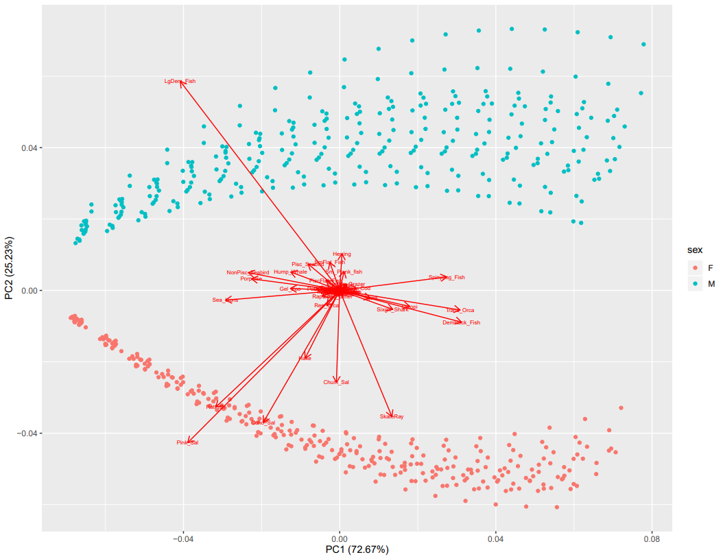
Fig. 1- Impact on prey of male and female harbor seals.
This is an early graph; some labels are difficult to read but still informative. Male impact is shown in blue; female, red. The x axis is mostly the sex ratio, higher biomass proportion for each sex on the right and lower on the left. The main drivers for the pattern appear to be large demersal fish, pink salmon, coho salmon, and ratfish. This is really cool since there is a clear separation in the sex impact and I can make inferences about the groups most impacted by sex ratio.
I’m happy with this graph but I was also interested in how this compares to different predators. I chose the sea lion group, since they are also pinnipeds and are abundant in the study area.
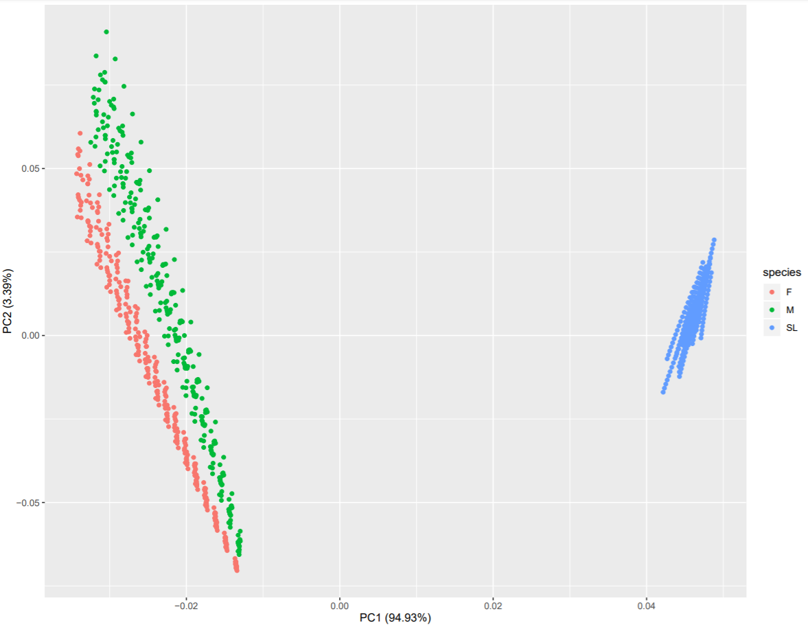
Fig. 2- Impact of prey for male and female harbor seals
relative to other predators.
Again, labels are a little small but male seals are in green; female, red; sea lions, blue. This graph not only informs about how harbor seal impact differs from other predators but also that the other predator’s impact is also changing with harbor seal sex ratio. There are some clear straight lines in the sea lion impact, these are the 17 sex ratios of each of the 20 models graphed here. It also shows the expected distribution of impacts for another predator. Clearly the harbor seal impact in the model varies much more than a group whose parameters are constant.
The multivariant approach seems to be working well and I look forward to using different tools and methods to get as much information from these models as I can. I also plan to include the fishery take from the model in January which shouldn’t change the effects too much but may change which species are driving the separation the most.
December Blog
Nathan Guilford, graduate student
1 January 2020
Earlier this month I was very excited to receive my sequence data for my 13 samples from the sequencing facility, with all samples providing good quality reads according to my initial QC! When I started digging into these samples, I received word from the facility that due to a lower than expected yield, they would have to re-run my samples. While at first this seemed like another delay in my results, I am glad they are attempting to achieve higher yields. Plus, I now have a practice data set to toy around with and pass through some various pipelines. A promising initial finding was that the samples on average had ~32% of their reads map to the harbor seal genome, meaning we did indeed have seal DNA in the end! Not only was it present, but this looks comparable to the work done with baboon feces where the enrichment method we used was created, which saw ~28% of the final reads map to a reference genome. This was just an average; some samples had mapping rates as high as 67%, while others were as low as 4%, highlighting the high variability we will most likely continue to see in these wild fecal samples due to unknown degradation rates.
Interestingly, the 4 samples that were mucous swabs from the surface of scat all had moderate rates from 21-33%, while the remaining samples comprised of scat slurries exhibited the full breadth of mapping rates. This may point towards the swabbing method as a more reliable seal DNA capture technique. This led me to question if the two collection methods would differ in the ability to capture prey sequences, a question which will require much more analysis, but one I wanted to quickly play with. I performed the same alignment process as above with each sample, however this time I used the Chinook salmon genome. Overall, there was a much lower average mapping rate of 2% ( 0.28% - 6.27% ), and neither collection method seemed to have a clear difference. Hopefully higher sequencing depths will capture more prey reads, and I can try other species/methods for prey identification/quantification.
As part of my project involves identifying variants (SNPs) within the seal genome for individual identification, I performed a variant analysis using the program ipyrad (an analysis toolkit for RADseq data). In these types of analyses, the parameters you initially set can have a large influence on your final variant panels, so I need to play around with these on my sample data set, using past literature and my specific project details to guide me. An initial analysis was able to identify SNPs between my samples, however the number was fairly low. Therefore, I am hoping that the re-run of my samples at the sequencing facility will significantly increase the depth of our sequencing, providing us not only with more reads for mapping to various reference genomes, but also for reliable SNP identification.
On another note, this month I was invited to attend the Seattle Aquarium’s alumni event, where previous volunteers/employees were able to present the work/research they have moved on to perform. This gave me the chance to see Hogan, the harbor seal who provided us with fecal samples for our genotyping controls. As you can see, he was very excited to hear about the project!
December Blog
Helen Krueger, undergraduate student
1 January 2020
This month I completed the first couple of steps of my research project. I collected wood samples from seal haul-outs in Whatcom Waterway. Took the samples back to the lab and cultured them, recording colony-forming units after 24 hours. I also found the dry sample weight and wet volume, in order to correct for differences in the amount of sample gathered. Sampling went smoothly. I had recruited a friend to help with the collection and be on the water with me, which ended up being a great idea because I failed to realize that scraping a log with a metal spoon is very difficult when you are in a floaty device that wants to push you away from your sampling site! My friend was able to push the nose of his kyake into mine so that I was stable enough to collect the samples. It was raining when we started sampling, but soon the sky opened up into a beautiful calm day.
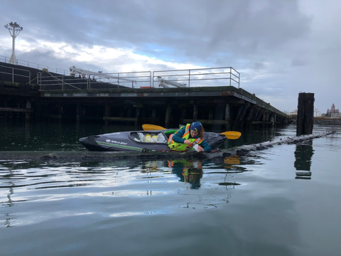
Image 1: Sampling day on the water in Whatcom Waterway. Photo
by J. Sayegh.
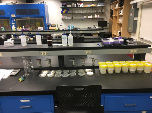
Image 2: All set up to culture my samples in the lab! Photo
by H. Krueger.
I have completed the first section of lab work, which is to culture the samples. The second step is to prepare the samples for SEM and use the SEM images to classify the bacteria. One of the main purposes of this taxonomic survey is to check for the presence or absence of pathogenic species. I hope to use the winter quarter to do all of this lab work and produce images to work with. Since I will be graduating in March, I would like to be completely done with the project as soon as possible and prepare my project poster for Scholars Week and the marine mammal conference. Since I have never done taxonomy on bacteria, I am unsure how time-intensive the process will be. Therefore the sooner I complete the lab work, the better shape I will be in. Happy 2020, all!
December Blog
Delaney Adams, undergraduate student
2 January 2020
The end of fall quarter provided a much needed break filled with lots of family time and relaxation at my home in Wichita, Kansas. I’ve been home for about three weeks now, and the time off has provided me with a chance to finally get caught up on all of the things I have been pushing off during the crazy, overbooked last couple of months. I’ve spent a large amount of time working on my introduction and outline for my project, as well as applying for jobs and preparing applications for thinking about the future. I have also finally had a chance to do more reading and research around my project, looking at cooperative hunting in Whatcom creek harbor seals.
While looking through materials, I came across a podcast about salmon abundance and how they might be interacting with other species in the Salish Sea, particularly the Southern Resident Killer Whales (SRKW). While not directly related to my project topic, I was excited to learn more. Dr. Greg Ruggerone, a natural resources consultant and salmon researcher, talks about how there is a distinct pattern of biannual abundance of Pink salmon due to their two-year life span in the North Pacific region that could be related to a biannual increased mortality rate of the SRKW that has been observed throughout the last 20 years (Neugebauer 2019). He discussed that in the 1990’s, there was a reduction of commercial harvest on chinook and pink salmon, and that led to a huge increase in the abundance of pink salmon, which feed on the same prey as juveniles in some regions. He hypothesizes that in the odd years, when there is a higher abundance of pink salmon, there is an interference with the SRKW that makes it more difficult for them to find their preferred prey, Chinook. Since they are large mammals, it takes about a year for the negative impact to take effect, which is why we see the biannual increased mortality rate consistently occurring in even years (Neugebauer 2019). There are still lots of unanswered questions regarding why we see this pattern of increased mortality in the SRKW population, but I enjoyed learning about another perspective on why the population is in decline and what might be able to be done about it in the future.
References
- Neugebauer, W. (Host). (2019, August 7). Are Pink Salmon a Threat to Southern Resident Orcas? Salmon Scientist Dr. Greg Ruggerone weighs in. [Audio podcast].